
Architecture
Isolation-first security data platforms
The query that ruins an analyst's afternoon is almost never the one they typed. It is the scheduled detection job that fired on its period somewhere else on the same cluster, backed up behind a dozen of its siblings, and turned a sub-second hunt into a thirty-second wait. So the thing you actually have to design against is co-tenant load rather than raw data volume. The question that decides the topology, then, is whether your interactive and scheduled work share a host at all.
Reading time: 9 minutes. The load numbers below come from a first-party single-host bench I ran in the lab this spring. I want to be careful about what they prove, because the failure shape travels and the absolute coordinates do not.
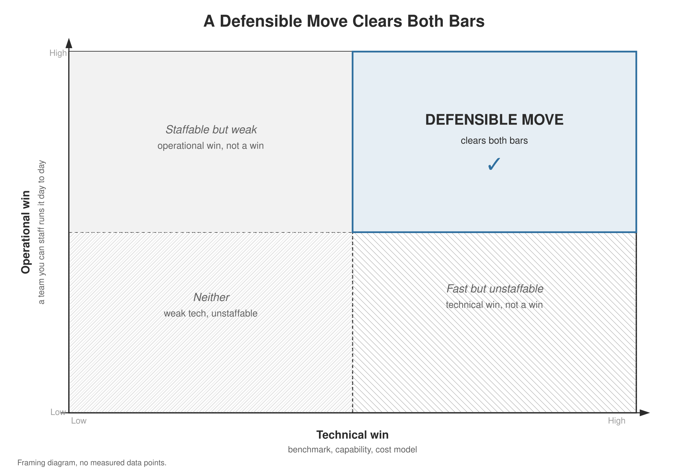
The wrong axis
Volume is the axis everyone benchmarks, and it is rarely the one that hurts.
Most security-data benchmarks I read measure one thing at a time. They take a single query, run it against a bigger and bigger corpus, and report how the latency grows. That is a useful number for sizing storage and picking a codec, but it tells you almost nothing about what an analyst experiences at two in the afternoon when the scheduled detection suite is also running. The interactive experience lives on a different axis, because the wait an analyst feels is set by who else is on the host and what they are doing. And that contention shows up long before the corpus gets large enough to matter on its own.
So I wanted to invert the usual test. Instead of asking how fast one query runs, I wanted to find the point where a steady background of scheduled detection jobs starts to ruin the foreground hunt, because that breaking point is the operational fact a SOC actually plans around. It is also the thing a winner-take-all latency chart hides completely. The interesting result is not which engine is fastest in a quiet room. It is how much company a fast engine tolerates before the interactive p95 falls off, and what the fall looks like when it comes.
The setup
One host, an interactive probe, and a scheduled load you turn up.
The bench runs on a single host, a Beelink with a Ryzen 5800H, under WSL2 with 48 GB and 14 threads. I split the cores deliberately with a cpuset that gives the engine twelve and the client two, so the client's own work does not masquerade as engine contention. One engine runs at a time against a 10-million-row connection-log corpus. The foreground is a small interactive probe whose latency I record against its intended send time rather than its start time, which keeps the slow tail honest under coordinated omission. The background is six pre-registered scheduled shapes on a 60-second cycle. The whole thing is open-loop, so when a scheduled response is slow the next one still fires on its period and the backlog grows. That is how a real scheduler behaves, where a closed-loop one would politely wait its turn.
The dial is demand, a multiple of the base scheduled rate that I turn up step by step. The question at each step is simple: has the interactive probe's p95 latency inflected yet. The baseline probe is noisy on its own, with a coefficient of variation in the 43.9 to 47.9 percent range. That is worth stating up front, because it sets how sharp an inflection has to be before I will call it a knee rather than noise. The pre-registration is strict about that: a knee counts only if it reproduces three times at the same step.
The finding
Flat through 32x, and then a knee at 64x
Three engines held the line in a way I did not expect to be this clean. ClickHouse reading its native tables, ClickHouse reading the same data over Iceberg, and StarRocks all kept the interactive p95 flat across the whole ladder up to 32x co-tenant scheduled load. And "flat" here is not a figure of speech, because just before the knee the p95 sat at roughly 0.099 seconds for ClickHouse native, 0.193 seconds for ClickHouse over Iceberg, and 0.112 seconds for StarRocks. A hundred-odd milliseconds at the ninety-fifth percentile, while a scheduled detection load thirty-two times the base rate runs in the background, is a quiet host.
Then at 64x the curve inflects sharply for all three, and the p95 jumps to about 3.21 seconds for ClickHouse native, 2.70 seconds for ClickHouse over Iceberg, and 3.77 seconds for StarRocks. That is a real knee, a sudden order-of-magnitude move that the prior steps gave no hint of. I reproduced it three times at the same step on every one of the three engines, 9 determinations out of 9, so it clears the pre-registration bar. The heights did not settle the same way. ClickHouse native came in between 3.11 and 3.47 seconds across those runs and StarRocks between 3.25 and 4.93, while ClickHouse over Iceberg spread widest of all, anywhere from 1.16 to 4.05 seconds at the knee, which is what saturation looks like up close. It is also why the claim is about where the knee sits and not how tall it is.
Breaking point · what reproduced
The part I keep coming back to is that even at the knee, none of these three crossed the lines that matter. The p95 at 64x ran roughly 2.7 to 3.8 seconds, which is over the sub-second floor an analyst would call snappy but still under the 10-second "flow" threshold where attention starts to break. It is well under the 30-second "tolerable" line too, past which people give up and go make coffee. So the headroom here is large relative to any scheduled detection load a real SOC would put on a single host. The inflection, when it finally comes, comes gracefully enough that you would notice it as a slowdown rather than an outage.
The caveat that travels
How far the 64x knee actually reaches
I want to be honest about how far this number reaches, because the temptation with a clean knee at 64x is to quote it like a spec, and it is not one. This is a single host with a fixed cpuset and a particular corpus, so the absolute coordinate, that 64x, is bound to those choices. It would not survive being copied onto a different machine with a different split and a heavier dataset. A larger corpus or heavier scheduled shapes moves the knee left, probably substantially, because the contention that produces it is throughput-determined and a bigger workload reaches saturation sooner. What travels from this bench is the ordering of the engines and the shape of the failure. These columnar/MPP engines stay flat and then inflect sharply rather than degrading linearly, and the inflection is a scheduler-saturation event you can see coming in the utilization counter. The exact step where it happens is yours to measure on your own host.
That distinction is the whole reason I prefer a breaking-point bench to a winner bench. A winner bench tells you which engine posted the lowest number in a quiet room, which is the least operationally useful fact you can collect. But a breaking-point bench tells you the shape of the cliff and roughly where it sits, which is what you actually plan capacity against. The number you carry home is that this class of engine holds flat under heavy co-tenant load and then knees, so size for the knee and leave margin.
Why isolation
The knee is the failure a dedicated deployment is built to avoid.
Once you see the load on the right axis, the case for an isolation-first platform stops being an aesthetic preference and turns into a capacity argument. If interactive and scheduled work share a host, then every analyst hunt is competing for the same cores as the detection suite. The headroom between you and the knee becomes a shared budget that someone else's scheduled job can spend without asking. When you isolate the interactive path onto its own deployment, the guarantee you are buying is that the foreground experience stays yours alone, because no scheduled backlog elsewhere can walk you up toward an inflection you did not provision for.
This bench is one way of stating why keeping interactive serving off heavy batch and scheduled compute is a standing architectural choice rather than a tuning afterthought. It matters most for a SOC that lives with the steady, always-on detection schedules this bench is meant to model.
The benchmark's good news is that the engines have more tolerance for company than I assumed, since three of them rode 32x of co-tenant scheduled load with the interactive p95 barely moving. So isolation is not always mandatory, and a small or moderate SOC may well be fine sharing a host. The benchmark's warning is that the tolerance is finite and the boundary is a knee rather than a gentle slope. So the moment your scheduled load grows, or your corpus does, or your shapes get heavier, the margin you were relying on shrinks. The inflection arrives sooner than the flat early steps would have led you to guess. Isolation-first is the posture that makes that arrival a non-event, because the job that would have spent your headroom is running somewhere you do not have to share.
On cost
What isolation costs, directionally
I am not going to put a TCO multiple on isolation, because I do not have a measured one and the figures that float around for "dedicated versus shared" tend to come from vendor decks rather than benches. Directionally, and only directionally, an isolated interactive deployment costs more in standing infrastructure than co-locating everything on one cluster, because you are provisioning a path that sits underused whenever the analysts are quiet. What you get back is harder to put on a spreadsheet: the absence of the afternoon where a scheduled backlog turned every hunt into a thirty-second wait, the analyst hours not lost to a slow console, the incident not investigated slowly because the platform chose that moment to inflect. Whether that trade pays depends on how much scheduled load you actually run and how much an interactive stall costs your team. That is the sort of thing you should size against your own knee rather than against a borrowed ratio. Treat any number you have seen for the cost of isolation, including the absence of one here, as illustrative until you have measured your own.
Takeaways
What to carry home.
- Benchmark the axis that hurts. Co-tenant scheduled load is what breaks the interactive experience, so a single-query-bigger-corpus chart misses the failure mode that actually shows up in production.
- These engines have real headroom. ClickHouse native, ClickHouse over Iceberg, and StarRocks held interactive p95 flat through 32x scheduled load on a single host before inflecting. Even at the 64x knee the p95 stayed under the 10-second flow line.
- The boundary behaves like a knee rather than a gentle slope, and the early flat steps give no warning. So plan for a sharp inflection and watch the utilization counter, which climbs a step ahead of the latency.
- Port the shape, not the coordinate. The 64x figure rides with this host, cpuset, and corpus; a larger corpus or heavier shapes moves it left, so measure your own knee and size to it.
- What isolation buys is a guarantee rather than raw speed, because a dedicated interactive deployment keeps a scheduled backlog elsewhere from spending the headroom you provisioned, which is the failure the knee represents.
Source data
The measurements here come from the SDW Lab workload-interferencebenchmark, specifically workload-interference/results/RESULTS.md for the per-step ladder and workload-interference/PHASE-C-SUMMARY.json for the reproduction. The knee this essay turns on hard-breaks on resource at 64× the base scheduled rate, and it is the Phase-C file that records the three repeat runs: knee_per_run comes back 64× on every arm, with the p95 band at that step kept separate from it, because the location reproduced and the height did not. The sibling results/results.json still carries a knee.reproduced field left over from the single-run Phase-B pass, which Phase C supersedes. Tier B, single host, one engine at a time, with a null-load calibration gate the run had to pass first.
